[en] Introduction to rainette
Julien Barnier
2026-05-05
Source:vignettes/introduction_en.Rmd
introduction_en.RmdCorpus preparation
For a description of the Reinert clustering method and its
implementation in rainette, please see the algorithms description vignette.
Split corpus into segments
As it doesn’t take into account terms frequencies but only there presence / absence, and as it assigns each document to only one cluster, the Reinert method must be applied to short and “homogeneous” documents. It could be ok if you work on tweets or short answers to a specific question, but with longer documents they must first be split into short textual segments.
You can use the split_segments() function for that, and
it can be applied directly on a tm or quanteda
corpus. In this article we will apply it to the sample
data_corpus_inaugural corpus provided by
quanteda.
library(quanteda)
library(rainette)

## Split documents into segments
corpus <- split_segments(data_corpus_inaugural, segment_size = 40)
split_segments will split the original texts into
smaller chunks, attempting to respect sentences and punctuation when
possible. The function takes two arguments :
-
segment_size: the preferred segment size, in words -
segment_size_window: the “window” into which looking for the best segment split, in words. IfNULL, it is set to0.4 * segment_size.
The result of the function is a quanteda corpus, which
keeps the original corpus metadata and adds an additional
segment_source variable, which keeps track of which segment
belongs to which document.
corpus## Corpus consisting of 3,658 documents and 5 docvars.
## 1789-Washington_1 :
## "Fellow-Citizens of the Senate and of the House of Representa..."
##
## 1789-Washington_2 :
## "On the one hand, I was summoned by my Country, whose voice I..."
##
## 1789-Washington_3 :
## "as the asylum of my declining years - a retreat which was re..."
##
## 1789-Washington_4 :
## "On the other hand, the magnitude and difficulty of the trust..."
##
## 1789-Washington_5 :
## "could not but overwhelm with despondence one who (inheriting..."
##
## 1789-Washington_6 :
## "In this conflict of emotions all I dare aver is that it has ..."
##
## [ reached max_ndoc ... 3,652 more documents ]## Year President FirstName Party segment_source
## 1 1789 Washington George none 1789-Washington
## 2 1789 Washington George none 1789-Washington
## 3 1789 Washington George none 1789-Washington
## 4 1789 Washington George none 1789-Washington
## 5 1789 Washington George none 1789-Washington
## 6 1789 Washington George none 1789-Washingtondfm computation
The next step is to compute the document-feature matrix. As our
corpus object is a quanteda corpus, we can
tokenize it and then use the dfm() function.
tok <- tokens(corpus, remove_punct = TRUE)
tok <- tokens_tolower(tok)
tok <- tokens_remove(tok, stopwords("en"))
dtm <- dfm(tok)
We also filter out terms that appear in less than 10 segments by
using dfm_trim.
dtm <- dfm_trim(dtm, min_docfreq = 10)Simple clustering
We are now ready to compute a simple Reinert clustering by using the
rainette() function. Its main arguments are :
-
k: the number of clusters to compute. -
min_segment_size: the minimum number of terms in each segment. If a segment contains less than this number of terms, it will be merged with the following or previous one if they come from the same source document. The default value is 0, ie no merging is done. -
min_split_members: if a cluster is smaller than this value, it won’t be split afterwards (default : 5).
Here we will compute 5 clusters with a min_segment_size
of 15 :
res <- rainette(dtm, k = 5, min_segment_size = 15)To help exploring the clustering results, rainette
provides an interactive interface which can be launched with
rainette_explor() :
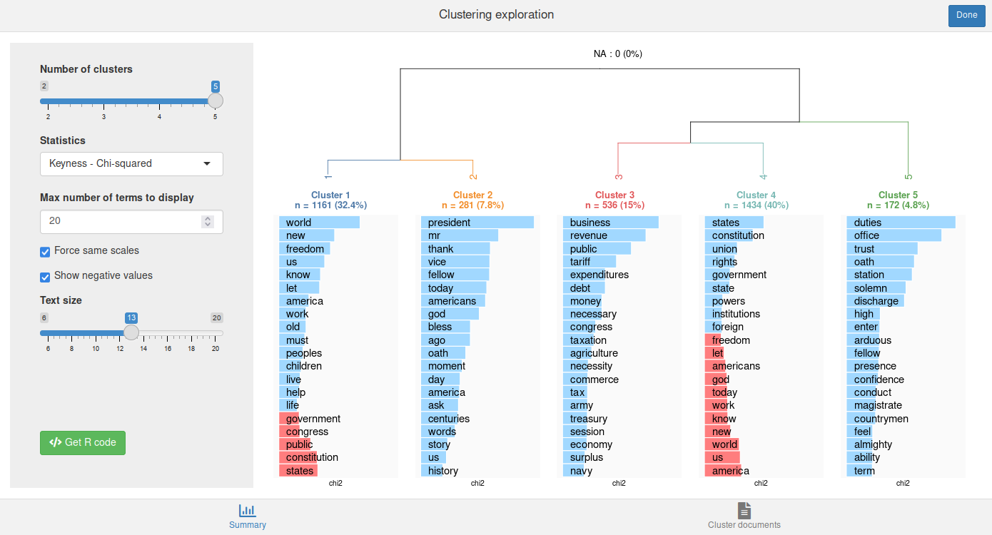
rainette_explor(res, dtm, corpus)
The interface allows to change the number of clusters, the displayed statistic, etc., and see the result in real time. By default the most specific terms are displayed with a blue bar or a red one for those with a negative keyness (if Show negative values has been checked).
You can also click on the Get R code button to get the R code to reproduce the current plot and to compute cluster membership.
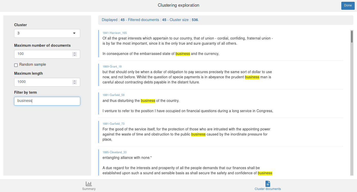
The Cluster documents tab allows to browse the documents from a given cluster. You can filter them by giving a term or a regular expression in the Filter by term field :

You can use cutree to get each document cluster at level
k :
cluster <- cutree(res, k = 5)This vector can be used, for example, as a new corpus metadata variable :
##   Year  President FirstName Party  segment_source cluster
## 1 1789 Washington    George  none 1789-Washington       4
## 2 1789 Washington    George  none 1789-Washington       4
## 3 1789 Washington    George  none 1789-Washington       5
## 4 1789 Washington    George  none 1789-Washington       5
## 5 1789 Washington    George  none 1789-Washington       3
## 6 1789 Washington    George  none 1789-Washington       3
Here, the clusters have been assigned to the segments, not to the
original documents as a whole. The clusters_by_doc_table
allows to display, for each original document, the number of segment
belonging to each cluster :
clusters_by_doc_table(corpus, clust_var = "cluster")## # A tibble: 60 × 6
## doc_id clust_1 clust_2 clust_3 clust_4 clust_5
## <chr> <int> <int> <int> <int> <int>
## 1 1789-Washington 0 0 6 29 2
## 2 1793-Washington 0 0 4 0 0
## 3 1797-Adams 0 8 2 46 3
## 4 1801-Jefferson 0 18 2 22 2
## 5 1805-Jefferson 0 5 3 43 6
## 6 1809-Madison 0 0 7 17 4
## 7 1813-Madison 0 5 3 23 2
## 8 1817-Monroe 0 3 10 61 14
## 9 1821-Monroe 0 2 10 72 31
## 10 1825-Adams 0 10 8 49 10
## # ℹ 50 more rowsBy adding prop = TRUE, the same table is displayed with
row percentages :
clusters_by_doc_table(corpus, clust_var = "cluster", prop = TRUE)## # A tibble: 60 × 6
## doc_id clust_1 clust_2 clust_3 clust_4 clust_5
## <chr> <dbl> <dbl> <dbl> <dbl> <dbl>
## 1 1789-Washington 0 0 16.2 78.4 5.41
## 2 1793-Washington 0 0 100 0 0
## 3 1797-Adams 0 13.6 3.39 78.0 5.08
## 4 1801-Jefferson 0 40.9 4.55 50 4.55
## 5 1805-Jefferson 0 8.77 5.26 75.4 10.5
## 6 1809-Madison 0 0 25 60.7 14.3
## 7 1813-Madison 0 15.2 9.09 69.7 6.06
## 8 1817-Monroe 0 3.41 11.4 69.3 15.9
## 9 1821-Monroe 0 1.74 8.70 62.6 27.0
## 10 1825-Adams 0 13.0 10.4 63.6 13.0
## # ℹ 50 more rowsConversely, the docs_by_cluster_table allows to display,
for each cluster, the number and proportion of original document
including at least one segment of this cluster :
docs_by_cluster_table(corpus, clust_var = "cluster")## # A tibble: 5 × 3
## cluster n `%`
## <chr> <int> <dbl>
## 1 clust_1 14 23.3
## 2 clust_2 55 91.7
## 3 clust_3 33 55
## 4 clust_4 44 73.3
## 5 clust_5 38 63.3Double clustering
rainette also provides a “double clustering” algorithm,
as described in the algorithms
description vignette : two simple clusterings are computed with
different min_segment_size values, and then crossed
together to get more robust clusters.
This can be done with the rainette2() function, which
can be applied to two already computed simple clusterings. Here, we
compute them with min_segment_size at 10 and 15.
res1 <- rainette(dtm, k = 5, min_segment_size = 10)
res2 <- rainette(dtm, k = 5, min_segment_size = 15)
We then use rainette2() to combine them. The
max_k argument is used to specify the maximum number of
clusters.
res <- rainette2(res1, res2, max_k = 5)One important argument of rainette2() is the
full argument :
- If
full = TRUE(the default), the best crossed clusters partition selection is made by keeping all non empty crossed clusters. This allows an exhaustive search and to identify the partition either with the highest sum of association χ², or the one with the highest total size. However, computation times can rise rapidly with the number of clusters. - If
full = FALSE, only the crossed clusters whose clusters are the most mutually associated are kept. Computations are much faster, but the highest k level with available partitions may be lower, and only the partitions with the highest association χ² values can be identified.
To be noted : with full = TRUE, if runtime is too high
you can add the parallel = TRUE argument to paralellise
some computations (won’t work on Windows, though, and may use much more
RAM).
In both cases, the resulting object is a tibble with, for
each level k, the optimal partitions and their characteristics.
Another interactive interface is available to explore the results. It is
launched with rainette2_explor().
rainette2_explor(res, dtm, corpus)
The interface is very similar to the previous one, except there is no
dendrogram anymore, but a single barplot of cluster sizes instead. Be
careful of the number of NA (not assigned segments), as it
can be quite high.
If some points are not assigned to any cluster, you can use
rainette2_complete_groups() to assign them to the nearest
one by using a k-nearest-neighbors algorithm (with k=1).
However this may not be recommended as you would then loose the
“robustness” of the new clusters computed by
rainette2().
clusters <- cutree(res, k = 5)
clusters_completed <- rainette2_complete_groups(dtm, clusters)